This page of the lesson is devoted to explaining the underlying mechanism of orbit traps. If you don’t care or find this too confusing, just proceed to the next page. This explanation provides motivation behind why we change certain parameters and may help you understand the effect these parameters have on the final image.
All fractal images in Fractal Domains are generated through a process of iteration (meaning repetition). For each point in the plane, a mathematical function is applied repeatedly. The effect of the mathematical function is to map the point into another point. The function is then applied to the new point to get yet another point. The process is illustrated in Figure 1 below. We start with the point labeled “0.” Applying the function yields the point labeled “1.” We apply the function again to point 1 to get point 2. This is done over and over until the point satisfies some escape criterion (usually, when the point gets past a
certain distance from the origin.)
The set of points that is generated by the iteration of the function starting from point 0 is called an “orbit.” In creating images, the point 0 is usually assigned a color based on some property of its orbit; very commonly, the color is determined by the number of points in the orbit, that is, the number of times the function is iterated before the escape criterion is satisfied.


An orbit trap is a geometrical shape usually centered at the origin. In Figure 2, the gray outline of a cross is the orbit trap. Now, as we iterate our function starting at point 0, we examine each point the orbit to see if it falls with the boundaries of the orbit trap. If any point falls within the boundaries we say it is “trapped” (hence the term “orbit trap”). In figure 2, one point in the orbit — point 5 — is trapped by the orbit trap.
When this occurs, we assign a color based on the place within the orbit trap the trapped point fell. For instance, a common thing to do for the cross orbit trap is to assign a color from a gradient map based on the distance from the nearest axis.[Of course, it is possible for more than one point in an orbit to be trapped in the orbit trap. Fractal Domains has several selectable strategies for dealing with this case, but we won’t discuss them at this point.]
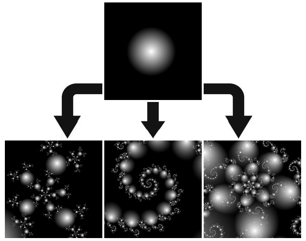
The effect of the orbit trap method of coloring points is to create a series of distorted “images” of the original orbit trap shape. These images are smaller copies, rotated and distorted, of the original shape. There are generally an infinite number of these images, reproduced at increasingly smaller scales. The exact appearance of these “echo” images depends on the particular mathematical function being used and which part of the plane is magnified.
The figure below illustrates this for the cross orbit trap and gives a modest example of the variety possible. The image at the top shows the original orbit trap, with the part of the cross that follows the real axis colored with a blue gradient and the part of the cross that follows the imaginary axis colored with a red gradient. When using this coloring scheme, an appearance of three-dimensional cylinders is created, but this is an illusion. The branches of the cross are simply colored by assigning each point a darker or lighter shade of red or blue depending on the point’s distance from the axis.
Below this image are three examples of how the original cross image becomes reproduced as extremely distorted copies of the original. These distorted shapes were dubbed “stalks” by Clifford Pickover when he discovered this phenomenon. (As far as I know, Pickover did not use gradients to get a 3D effect in his stalk images, though — he used black on a white background [see, for example, Pickover, “Computers, Patterns, Chaos and Beauty”, 1990, St. Martin’s Press]. The use of gradients for a 3D effect, as well as the generalization from a cross-shaped trap to arbitrary shapes, was developed by Paul Carlson.)

In the figure below, we show what happens when a different shape is used as an orbit trap. Now we use a circle about the origin as the orbit trap and we use a gradient coloring based on the distance from the origin. Again we use a gradient, this time a gray scale gradient based on the distance from the center of the circle. This gives the circle the appearance of a sphere.